Inspired by the cooking videos of the format "n levels of [dish]", I’m here
applying a similar concept to scientific modeling. I will be comparing 4
levels of projectile motion, from the easiest "textbook" model, which is
the simplest of all and assumes only constant gravity in a flat Earth,
to a more complex model taking into account factors like quadratic drag,
buoyancy, and the Magnus effect.
Level 1: just
constant gravity in a vacuum
This is the easiest level of all. It is ubiquitous in all middle and
high school level textbooks on physics (Serway & Jewett, 2016), and it’s commonly used as a way
to teach the basic idea of 2D kinematics, and tracking the position as a
function of time of an object in the ℝ2 plane using parametric
equations of the form x = f(t), y = g(t).
Considering gravity in the negative y direction to be the only force
acting on the object, and, as Galileo noticed, if gravity is the only
force on an object, the mass is not involved in the motion. We assume
the object is significantly close to Earth’s surface, in which case
constant gravity in a single direction can be assumed. With all of this
information, Newton’s second law gives the simple equations $$\begin{align}
\ddot{x}=0,
\\
\ddot{y}=-g
\end{align}$$ where g = 9.8 m/s2 is the
standard Earth surface gravity. These equations are the "trivial" kind
of ODE, in which simply integrating both sides twice suffices to solve
them. Assuming the particle begins with initial speed u at the origin, the solutions are
simply $$\begin{align}
x(t) = ut \cos \theta,
\\
y(t) = ut\sin \theta - \frac{1}{2}gt^2,
\end{align}$$ where θ
is the angle of launch with respect to the horizontal. Eliminating t, the trajectory can be easily
found to be $$y=x\tan(\theta)-\frac{gx^2}{2u^2\cos^2(\theta)},$$
which is a parabola, with an inverse "U" shape in the xy plane. From this the
range, the area swept and more can be computed. This case won’t be
discussed further here, as the reader is most likely familiar with the
dynamics, which they almost certainly covered in their secondary school
education. This case is covered with detail in introductory books like
(Serway & Jewett, 2016) (Knight, 2008).
Level 2:
constant gravity with a linear drag force
Finding a theoretical formula for the drag force is a well-known
problem in fluid mechanics, that notoriously requires heavy usage of
experimental and numerical rather than pure analytic methods. However,
for low Reynolds numbers (Re < 1),
there exists a very simple solution for the drag as a function of the
speed v (Acheson, 2005). It is known as Stokes’ law,
and it is a relation of the form F = −bv, where,
e.g., in the case of a sphere of radius r, b = 6πηr,
where η is the viscosity of
the medium. This is the most complex case that admits a closed form
analytical solution (Taylor, 2005). The net force acting on the object in
this case is F = −mgĵ − bv.
So, resolving the resulting equation of motion into the x and y components gives $$\begin{align}
m\ddot{x}=-b\dot{x}
\\
m\ddot{y}=-mg-b\dot{y}
\end{align}$$ These equations can be solved through
separation of variables, or via the general theory of linear constant
coefficient 2nd order differential equations (Logan, 2015). Either way, the solutions are found to
be $$\begin{align}
x(t)=\frac{mv_x(0)}{b}(1-e^{-\frac{bt}{m}})
\\
y(t)=\bigg( \frac{mg}{b} + v_y(0))\bigg
)\frac{m}{b}(1-e^{-\frac{bt}{m}})-\frac{mgt}{b}.
\end{align}$$ These solutions imply that the projectile
travels through a parabola-like curve that becomes steeper as the
projectile gets closer to the ground. A trajectory equation similar to
(3) can be found by eliminating t from equations (5), or
alternatively, via a differential equation (Borghi, 2013): $$y=\frac{v_y(0)+v_{\mathrm{T}}}{v_x(0)}x+\frac{m^2g}{b^2}\ln\bigg(
1-\frac{mx}{bv_x(0)} \bigg),$$ where $v_\mathrm{T}=\frac{mg}{b}$. In this case,
there is no general closed form analytical solution for the drag and it
must be computed either numerically via e.g., Newton’s method, or via
perturbations (Taylor, 2005).
This kind of equations should only be used in the physical world to
model e.g., the motion of a microscopic object like a bactetria. As with
the previous level, this case won’t be treated much further here, since
it is a standard problem in undergraduate level textbooks (Taylor, 2005) (Greiner, 2004)
Level 3:
constant gravity with a quadratic drag force
We now begin to examine the most realistic models. We’re now entering
into terrain where there’s no general closed form analytical solution,
though (Parker, 1977) gives some
approximate analytical solutions for both the the short and long time
regimes. I will present some Python code with the numerical
integrations. In this case, the force acting on the projectile is almost
the same in the previous section, but with the drag force instead being
Fdrag = −c|v|v.
In vector form, thus, the equations take the form $$m\ddot{\mathbf{r}}=-mg\hat{j}-c|\dot{\mathbf{r}}|\dot{\mathbf{r}}.$$
Which in terms of components, turns into $$\begin{align}
m\ddot{x}=-c\dot{x}\sqrt{\dot{x}^2+\dot{y}^2}
\\
m\ddot{y}=-mg-c\dot{y}\sqrt{\dot{x}^2+\dot{y}^2}.
\end{align}$$ These equations are now coupled and non-linear,
making a general closed form analytical solution impossible. Highly
accurate approximations for the maximum height, arrival time, and flight
range are given in (Turkyilmazoglu, 2016). As per the so-called "drag
equation", the coefficient c
can be found to be $c=\frac{1}{2}C_d
A\rho$, where Cd is the
so-called "drag coefficient", A is the cross-sectional area and
ρ is the density of the
medium. To visualize this case, it’s better to proceed with an example.
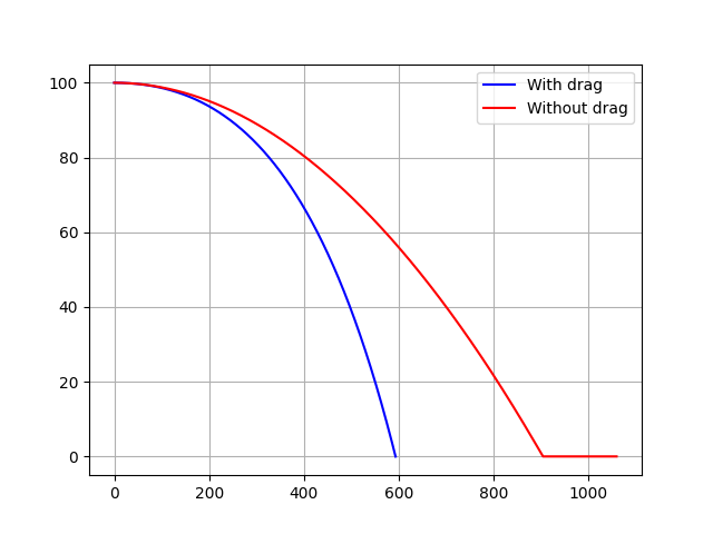
Here, we’ll procede with a horizontal throw case application of
equations (8). We will model a cannon ball with density ρb = 707 kg/m3,
corresponding to the density of certain kinds of stone, and a radius of
18.25 cm. Here’s the plotted trajectory of a sample numerical
integration of equations with time step h = 0.001 (8) in Python with Heun’s
method, a second order method (Süli, 2003):
This image shows the path equations (8) predict for a particle initially
at rest along the vertical direction, starting from x(0) = 0, y(0) = 100 m and u = 200 m/s. The image is then
compared with what would the path been like without drag. One of the
things we can notice from the image is that the path of the particle
with drag is steeper than the path without drag. Also, that the range
has been significantly reduced, the particle without drag goes farther
than the one with drag. This happens because the drag reduces the
velocity of the particle as time passes. It can be seen from equations
(8) that if the velocity is always positive, the acceleration will
always be positive, meaning the velocity is always decreasing in both
the x and y directions. The model presented in
this section is good for Reynolds numbers Re > 1000.
Level
4: Constant gravity with quadratic drag, buoyancy, Magnus force
This level is the most realistic out of the ones presented so far. It
still models the behavior with a deterministic differential equation,
but takes the Magnus force into account. Aditionally, this model is now
3D. Applications of this model include sports. For example, it’s useful
to model the dynamics of a ball after a footballer kicks a penalty, both
the trajectory and where it ends up landing, as a result of simply the
initial kick the footballer gives. Making it therefore useful, e.g., in
game development to make FIFA/PES-like games. The mass here is treated
like a rigid body. Therefore, these equations, properly speaking, track
the trajectory of the center-of-mass of the ball. The Magnus force
acting on a given object can be modeled by a simple expression: FMagnus = Sω × v
(Fitzpatrick, 2004). Experiments
to determine the value of the Magnus force coefficient expression are
given in (Goff, 2013). We can
also add buoyancy here. It also has a simple expression, the buoyant
force is the removed mass times the gravitational acceleration: Fb = −ρfVgk̂.
Combining all of this gives the equation: $$m\ddot{\mathbf{r}}=-mg\hat{k}+\rho_b
Vg\hat{k}-c|\dot{\mathbf{r}}|\dot{\mathbf{r}}+S\mathbf{\omega}\times\mathbf{\dot{\mathbf{r}}}.$$
Like in the previous section, we can divide this into components, though
this time there are 3 of them: $$\begin{align}
m\ddot{x}=-c\dot{x}\sqrt{\dot{x}^2+\dot{y}^2+\dot{z}^2}-S\omega\dot{y}
\\
m\ddot{y}=-c\dot{y}\sqrt{\dot{x}^2+\dot{y}^2+\dot{z}^2}+S\omega\dot{x}
\\
m\ddot{z}=g\bigg(\frac{\rho_f
V}{m}-1\bigg)-c\dot{z}\sqrt{\dot{x}^2+\dot{y}^2+\dot{z}^2}
\end{align}$$ Like in the previous case, an analytical
solution is impossible. Though it’s possible to derive asymptotic
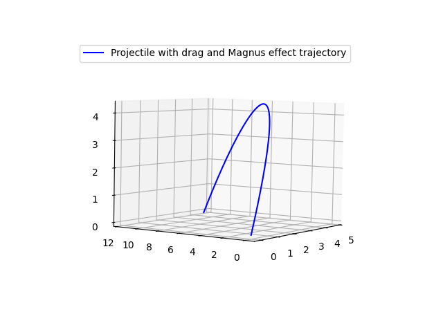
special cases from this equation, as done in (Turkyilmazoglu, 2020). This is what a python script
solving equations (10) numerically with initial conditions x(0) = y(0) = z(0) = 0
and ẋ(0) = 7 m/s, ẏ(0) = 5 m/s, ż(0) = 10 m/s, for a football with a
mass of 450 g, and a radius of 11.15 cm:
This shows how the trajectory is deviated horizontally thanks to the
Magnus force, as well as of course the steeper trajectory derived from
the drag force. In this case, the numerical integration took the time
step h = 0.01, and took a
total of 10000 steps to produce this figure. It’s interesting to note
how the Magnus force has a similar form to the magnetic force F = qv × B,
making this Magnus force mimick the effect a magnetic field has over a
charged particle.
Discussion
In this pedagogical paper, we have revised 4 different levels of
complexity for the projectile motion physical problem. We have increased
our complexity from the easiest, textbook model that is simple but
unrealistic in many cases to the most complex model that describes more
things accurately, e.g., a football’s trajectory after a penalty is
taken. This paper shows how can complex phenomena be modeled, and how
models take into account more and more variables as the physical world
demands it.
References
Serway, R. A., Jewett, J. W. Physics for
Scientists and Engineers. Cengage Learning, Boston, MA, 9th
edition, 2016
Knight, R. D. Physics for Scientists and Engineers, a
strategic approach. Addison Wesley, San Francisco, CA, 2nd edition,
2008
Acheson, D. J. Elementary Fluid Dynamics. Oxford
University Press, Oxford, England, 2005
Taylor, J. R. Classical
Mechanics. University Science Books, Melville, CA, 2005
Logan, J.
D. A First Course in Differential Equations. Springer,
Switzerland, 2015
Borghi, R. Trajectory of a body in a resistant medium:
an elementary derivation. European Journal of Physics,
34, 359-369, 2013
Greiner, W. Classical Mechanics: Point
Particles and Relativity, Springer, New York, NY, 2004
Parker, G.
W. Projectile motion with air resistance quadratic in the speed.
American Journal of Physics45(7), 606-610, 1977
Turkyilmazoglu, M. Highly accurate analytic formulae for projectile
motion subjected to quadratic drag. European Journal of Physics37, 1-12, 2016
Süli, E., Mayers, D. F. An Introduction to
Numerical Analysis. Cambridge University Press, Cambridge, England.
2003
Fitzpatrick, R. Computational Physics: An introductory
course Author: Austin, TX. 2004
Goff, J. E. A review of recent
research into aerodynamics of sport projectiles. Sports
Engineering16, 137-154, 2013
Turkyilmazoglu, M.,
Altundag, T. Exact and approximate solutions to projectile motion in air
incorporating Magnus effect Eur. Phys. J. Plus 135:566,
2020